An introduction to `picreg`

Introduction

picreg is the R implementation of the Pivotal Information Criterion (PIC) developed by Sardy, van Cutsem, and van de Geer in https://arxiv.org/abs/2603.04172. PIC is a general framework to improve on BIC and LASSO for fitting sparse regression linear models in which the regularization parameter \lambda is selected automatically from a pivotal statistic. As a result, PIC removes the need for cross-validation and achieves more accurate support recovery by better identifying the true non-zero coefficients. The package fits the resulting estimators across six response distributions - Gaussian, binomial, Poisson, exponential, Gumbel, and Cox - combined with three sparsity-inducing penalties; \ell_1 (LASSO), the Smoothly Clipped Absolute Deviation (SCAD), and Minimax Concave Penalty (MCP).

Given data \mathcal{D} = (X, y), where X \in \mathbb{R}^{n \times p} denotes the design matrix and y \in \mathbb{R}^n the response vector, a base loss l_n(\boldsymbol{\theta}, \sigma; \mathcal{D}) = \frac{1}{n} \sum_{i=1}^n l(\theta_i, \sigma; \mathcal{D}) (with a possible nuisance parameter \sigma), and a sparsity-inducing penalty P (possibly non-convex), pic() minimizes the Pivotal Information Criterion (PIC) by solving \min_{\beta_0,\,\boldsymbol{\beta}}\left\{ \phi\bigl(l_n(\boldsymbol{\theta}, \sigma; \mathcal{D})\bigr) + \lambda_\alpha^{\mathrm{PDB}}\, P(\boldsymbol{\beta})\right\}, \qquad \boldsymbol{\theta} = g\bigl(\beta_0\mathbf{1} + X\boldsymbol{\beta}\bigr), where \lambda_\alpha^{\mathrm{PDB}} is the pre-fixed for the parameter \lambda chosen as the upper \alpha-quantile of a statistic \Lambda made pivotal with respect to unknown parameters \sigma,\, \beta_0 thanks to the distribution-specific pair (\phi,\, g).

Internally, picreg uses FISTA (Fast Iterative Soft-Thresholding Algorithm) as the optimization scheme.

Installation

picreg is available on CRAN:

install.packages("picreg")

Alternatively, the development version can be installed from GitHub:

# install.packages("remotes")
remotes::install_github("VcMaxouuu/picreg")

Once installed, load it with:

library(picreg)

Quick start

This section walks through the shared interface that all six distributions expose: fitting a model, inspecting it, predicting on new data, selecting the regularization parameter, and visualizing the relevant quantities. Distribution-specific tooling is deferred to the Generalised linear models section.

We illustrate the workflow on the default Gaussian distribution with the LASSO (\ell_1) penalty. The package ships a small synthetic dataset QuickStartExample (n = 100, p = 30, of which 5 active variables and 25 noise variables). Active columns are named gene_1, ..., gene_5 and noise columns noise_1, ..., noise_25.

data(QuickStartExample)
X <- QuickStartExample$X
y <- QuickStartExample$y

Fitting a model

The simplest call to pic() returns a fitted model with all defaults: Gaussian distribution, LASSO penalty, automatic PDB selection of \lambda:

fit <- pic(X, y)

These defaults can be overridden through two main arguments:

family: the response distribution: "gaussian" (default), "binomial", "poisson", "exponential", "gumbel", or "cox".
penalty: the sparsity-inducing penalty used during training: "lasso" (default), "scad", or "mcp".

Behind the scenes, pic() standardizes the columns of X to zero mean and unit variance, computes \lambda_\alpha^{\mathrm{PDB}}, and minimizes the objective with FISTA. A concise summary is available through the summary method:

summary(fit)

## pic fit summary
##   family    : gaussian
##   penalty   : lasso
##   lambda    : 0.311
##   dimensions: n = 100, p = 30
##   selected  : 5 / 30
##   intercept : 0.006603
## 
##   Non-zero coefficients (original scale):
##  variable coefficient
##    gene_3     -0.7508
##    gene_4     -0.6489
##    gene_1     -0.4028
##    gene_5      0.1380
##    gene_2     -0.0463

Inspecting the fit

The returned object carries everything needed for downstream analysis:

# Number of selected features and their identifiers
fit$df

## [1] 5

fit$selected

## [1] "gene_1" "gene_2" "gene_3" "gene_4" "gene_5"

# Selected regularization parameter
fit$lambda

## [1] 0.3109731

# Family and penalty descriptors
fit$family

## family: gaussian (link g = identity, phi = sqrt)

fit$penalty

## lasso()

When X is supplied as a data frame, or as a matrix carrying column names, picreg uses them throughout the output. As shown above, fit$selected returns the names of the selected variables rather than their integer indices. Bare matrices fall back to the default V1, ..., Vp naming.

Coefficients

The full coefficient vector is accessible either through fit$beta (standardized, numeric vector) or through coef(), which returns a one-column sparse matrix (class "dgCMatrix") on the original scale of X by default; zero coefficients are printed as .. Note that fit$beta is a bare numeric vector and carries no variable names, whereas coef() is more informative: it labels every coefficient with its variable name (and adds the "(Intercept)" row):

coef(fit)                          # original scale

## 31 x 1 sparse Matrix of class "dgCMatrix"
##             coefficient
## (Intercept)  0.00660255
## gene_1      -0.40277095
## noise_1      .         
## noise_2      .         
## noise_3      .         
## gene_2      -0.04628404
## noise_4      .         
## noise_5      .         
## noise_6      .         
## noise_7      .         
...

# coef(fit, standardized = TRUE)   # standardized scale; same as fit$beta

Predicting on new data

The user can make predictions from the fitted object using the predict() function. The primary argument is newx, a matrix of values for X at which predictions are desired. Two types are universally available: "link" (the linear predictor X\boldsymbol{\beta} + \beta_0) and "response" (the mean response g(\eta)). In the Gaussian case of course (since g is the identity), both types gives the same outputs. Binomial fits additionally accept type = "class" for hard label prediction.

predict(fit, newx = X[1:5,])                  # response

## [1]  0.4305631  1.8606175 -1.0359871  1.1197544  0.2146807

predict(fit, newx = X[1:5,], type = "link")   # linear predictor

## [1]  0.4305631  1.8606175 -1.0359871  1.1197544  0.2146807

Visualizing the fit

The standard plot method draws the non-zero coefficients in descending order of absolute magnitude:

plot(fit)

Each segment represents the value of one selected coefficient. The descending order makes the relative importance of the selected variables immediately visible. Passing standardized = FALSE rescales the displayed coefficients back to the original scale of X. In that case, differences in predictor scales may distort the relative magnitudes of the coefficients, so direct comparisons between them are generally no longer meaningful.

Selecting the regularization parameter

The parameter \lambda governs the trade-off between data fit and sparsity. pic() selects it automatically as \lambda=\lambda_\alpha^{\mathrm{PDB}}.

The selection of \lambda is calibrated such that, under the null hypothesis H_0:\boldsymbol{\beta} = \mathbf{0}, the estimated model that minimizes PIC returns no selected variables with high probability. To that aim, the pivotal detection boundary \lambda_\alpha^{\mathrm{PDB}} is defined as the upper \alpha-quantile of \Lambda=\left\lVert \nabla_{\boldsymbol\beta}\left(\phi\circ l_n\right) \left(g(\hat\beta_0\mathbf 1), \hat\sigma; (X, Y_0)\right) \right\rVert_\infty, that is, the gradient evaluated at \boldsymbol{\beta} = \mathbf{0} given data sampled under the null hypothesis Y_0. The nuisance parameters are set to their maximum-likelihood estimates. By default alpha = 0.05 in a pic() call. The quantile depends only on X, the underlying distribution family, and \alpha. It is independent of the observed response data y. As a result, the tuning-free parameter \lambda_\alpha^{\mathrm{PDB}} can be determined a priori.

Calculation methods

The quantile is calculated via one of three methods, set through the lambda_method argument of pic():

"mc_exact" (default). Distribution/family-aware Monte Carlo: for each of lambda_n_simu draw, a null response is sampled, the distribution-specific gradient is evaluated at \boldsymbol{\beta} = \mathbf{0}, and its supremum norm is recorded. The empirical (1-\alpha) quantile of the simulated norms is returned.
"mc_gaussian". Samples the gradient directly from its Gaussian CLT limit \mathcal{N}\bigl(0,\, c(n)\,\Sigma_X / n\bigr), with \Sigma_X = X^\top X / n and c(n) a distribution-specific scaling factor. Cheaper than "mc_exact" and essentially equivalent once n is moderately large.
"analytical". Closed-form Bonferroni bound, \Phi^{-1}\!\bigl(1 - \alpha / (2p)\bigr) \sqrt{c(n)/n}. Not based on a Monte-Carlo simulation, O(1), slightly conservative. Useful in ultra-high dimensions.

Visualizing the null distribution

Monte Carlo methods keep the simulated null statistics on the fit and can be visualized by calling plot() on fit$lambda_pdb. By default pic() uses lambda_n_simu = 2000 Monte-Carlo simulations.

plot(fit$lambda_pdb)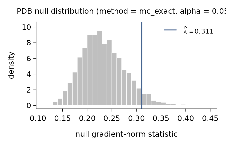

The histogram shows the empirical distribution of the null and the vertical line marks the selected \widehat{\lambda} at the (1-\alpha) quantile. A more detailed text summary is available through pdb_summary():

pdb_summary(fit)

## PDB lambda selector
## -------------------
##   method       : mc_exact
##   alpha        : 0.05
##   n_simu       : 2,000
##   lambda_hat   : 0.311
## 
##   Null distribution:
##    min     q05     q25  median     q75     q95     max  
## 0.1135  0.1656  0.2014  0.2283  0.2606  0.3108  0.4406  
## 
##   mean = 0.2326      sd = 0.0444

The "analytical" method has no simulated draw and therefore nothing to plot; pdb_summary() then reports only the selector metadata.

Supplying \lambda manually

A value of \lambda known in advance - from a previous fit, from theory, or to share the same regularization across penalties on the same dataset - can be supplied directly via the lambda argument of pic(). The PDB calibration is then skipped. This is particularly useful when comparing the three penalties (LASSO, SCAD, MCP) on the same problem, since the PDB choice of \lambda does not depend on the penalty itself.

fit_lasso <- pic(X, y, penalty = "lasso", lambda = fit$lambda)
fit_scad  <- pic(X, y, penalty = "scad",  lambda = fit$lambda)
fit_mcp   <- pic(X, y, penalty = "mcp",   lambda = fit$lambda)

data.frame(
  penalty = c("lasso", "scad", "mcp"),
  df      = c(fit_lasso$df, fit_scad$df, fit_mcp$df),
  lambda  = c(fit_lasso$lambda, fit_scad$lambda, fit_mcp$lambda)
)

##   penalty df    lambda
## 1   lasso  5 0.3109731
## 2    scad  5 0.3109731
## 3     mcp  5 0.3109731

Generalised linear models

The interface described in the Quick start applies unchanged to all six distributions. Each one is identified by a name string passed to family = and is characterized by the pair (\phi, g): \phi applied to the base loss, and g relating the linear predictor \eta = \beta_0 + X\boldsymbol{\beta} to the mean response.

Gaussian

"gaussian" is the default family argument for pic(). The objective function for the Gaussian distribution uses the MSE for l_n and \phi(\cdot) = \sqrt{\cdot}, g(\cdot) = \mathrm{Id} as transformations, resulting in the square-root LASSO objective \min_{\beta_0,\,\boldsymbol{\beta}}\left\{\sqrt{\frac1n\sum_{i=1}^n\left(y_i-(\beta_0+\mathbf x_i^T\boldsymbol\beta\right)^2} + \lambda_\alpha^{\mathrm{PDB}}\, P(\boldsymbol{\beta})\right\}. This is the canonical pivotal alternative to the standard squared loss: it makes the gradient at \boldsymbol{\beta} = 0 scale-free, so the PDB threshold does not require an estimate of the noise standard deviation.

Binomial

family = "binomial" is used for logistic regression when the responses y_i \in \{0, 1\} are binary. In this case, pic requires y to be a vector containing only 0 and 1 values. Any other format or values in y will return an error. picreg uses a variance-stabilized transformation of the Bernoulli likelihood. With \phi(\cdot) = \mathrm{Id} and the logistic link \theta_i = g(\eta_i) = (1 + e^{-\eta_i})^{-1}, pic(family = "binomial") minimizes \min_{\beta_0, \boldsymbol\beta}\left\{ \frac{1}{n}\sum_{i=1}^{n}\left( 2 y_i \sqrt{\tfrac{1 - \theta_i}{\theta_i}} + 2 (1 - y_i) \sqrt{\tfrac{\theta_i}{1 - \theta_i}} \right)+\lambda_\alpha^{\rm PBD}P(\boldsymbol\beta)\right\}, \qquad \theta_i = \frac{1}{1+\exp(-(\beta_0+\mathbf x_i^T\boldsymbol\beta))} The classical logistic link is preserved; only the loss itself is modified to obtain a pivotal gradient at the null.

data(BinomialExample)
X <- BinomialExample$X
y <- BinomialExample$y
fit_binom <- pic(X, y, family = 'binomial')
print(fit_binom)

## pic fit (pic.binomial)
##   family   : binomial
##   penalty  : lasso
##   lambda   : 0.191493
##   selected : 5 / 50
##   intercept: -0.281037

Binomial fits additionally support hard label prediction when passing type = "class" to the predict() function.

predict(fit_binom, newx = X[1:5, ], type = 'response')

## [1] 0.4193490 0.7368105 0.2277823 0.3310245 0.5189012

predict(fit_binom, newx = X[1:5, ], type = 'class')

## [1] 0 1 0 0 1

Poisson

For count responses y_i \in \mathbb{N}, the same pivotalization recipe is applied to the Poisson likelihood. With \phi(\cdot) = \mathrm{Id} and the canonical log link \theta_i = g(\eta_i) = e^{\eta_i}, pic(family = "poisson") minimizes \min_{\beta_0, \boldsymbol\beta}\left\{ \frac{1}{n}\sum_{i=1}^{n}\!\left( \frac{2 y_i}{\sqrt{\theta_i}} + 2 \sqrt{\theta_i} \right)+\lambda_\alpha^{\rm PDB}P(\boldsymbol\beta)\right\}, \qquad \theta_i = \exp(\beta_0+\mathbf x_i^T\boldsymbol\beta). The canonical log link is kept unchanged; the pivotal property is obtained through the loss rather than through the link. pic requires y to be a vector containing only non negative values.

Exponential

The standard Exponential negative log-likelihood is used directly, no transformation are needed. With \phi(\cdot) = \mathrm{Id} and \theta_i = g(\eta_i) = e^{\eta_i}, pic(family = "exponential") minimizes \min_{\beta_0, \boldsymbol\beta}\left\{ \frac{1}{n}\sum_{i=1}^{n}\left( \log{\theta_i} + \frac{y_i}{\theta_i} \right)+\lambda_\alpha^{\rm PDB}\right\}, \qquad \theta_i = \exp(\beta_0+\mathbf x_i^T\boldsymbol\beta). Again, pic requires y to be a vector containing only non negative values.

Gumbel

The Gumbel distribution targets location-scale models with extreme-value noise. The base log-likelihood is l_n(\boldsymbol{\theta}, \sigma) = \log(\sigma) + \frac{1}{n}\sum_{i=1}^{n} \bigl(z_i + e^{-z_i}\bigr), \qquad z_i = \frac{y_i - \theta_i}{\sigma}. With \phi(\cdot) = \exp(\cdot) and the identity link \theta_i = g(\eta_i) = \eta_i, the optimization objective is \phi\bigl(\ell_n(\boldsymbol{\theta}, \sigma; \mathcal{D})\bigr) = \exp\bigl(\ell_n(\boldsymbol{\theta}, \sigma)\bigr). The scale parameter \sigma is re-estimated internally by maximum likelihood at every iteration; the user does not pass it explicitly.

Cox

The Cox proportional-hazard model is the survival counterpart of the other GLMs. The response y must be a two-column matrix (t_i, \delta_i) of event times and event indicators (\delta_i = 1 if event, 0 if censored). With \phi(\cdot) = \sqrt{\cdot} and \theta_i = g(\eta_i) = \eta_i, pic(family = "cox") minimizes the square-root normalized partial log-likelihood: \min_{\boldsymbol\beta}\left\{ \sqrt{ -\frac1n\left( \sum_{i=1}^{n} \delta_i \eta_i - \sum_{i=1}^{n} \delta_i \log\left(\sum_{j \in R_i} e^{\eta_j}\right) \right)}+\lambda_\alpha^{\rm PDB}P(\boldsymbol\beta)\right\}, where R_i denotes the risk set at event time t_i. Breslow approximation for tied event times is used. When family = "cox" is used, pic automatically fits the model without an intercept.

The package ships a small survival dataset CoxExample (n = 250, p = 50, with 5 active variables and 45 noise variables) generated under an exponential proportional-hazards model with independent exponential censoring. The censoring rate is roughly 40\%. The response is a two-column matrix with columns time and event, the standard input format for family = "cox".

data(CoxExample)
X_cox <- CoxExample$X
y_cox <- CoxExample$y
print(y_cox[1:7, ])

##             time event
## [1,] 0.005565264     1
## [2,] 0.017211836     1
## [3,] 0.017762667     1
## [4,] 0.794925355     0
## [5,] 0.008978275     1
## [6,] 0.123304085     1
## [7,] 0.179501892     0

fit_cox <- pic(X_cox, y_cox, family = "cox")
print(fit_cox)

## pic fit (pic.cox)
##   family   : cox
##   penalty  : lasso
##   lambda   : 0.0476666
##   selected : 5 / 50

In addition to the shared interface, pic.cox objects carry the Breslow estimates of the baseline cumulative hazard H_0(t) and the baseline survival S_0(t) = \exp\!\bigl(-H_0(t)\bigr), accessible directly through fit_cox$baseline_cumulative_hazard and fit_cox$baseline_survival. They are also visualized through plot_baseline():

plot_baseline(fit_cox)

For any new design, predict_survival_function() returns the common time grid and a matrix of survival probabilities, one column per subject. The result is plotted directly with plot_survival_curves():

sf <- predict_survival_function(fit_cox, newx = X_cox[1:3, ])
plot_survival_curves(sf)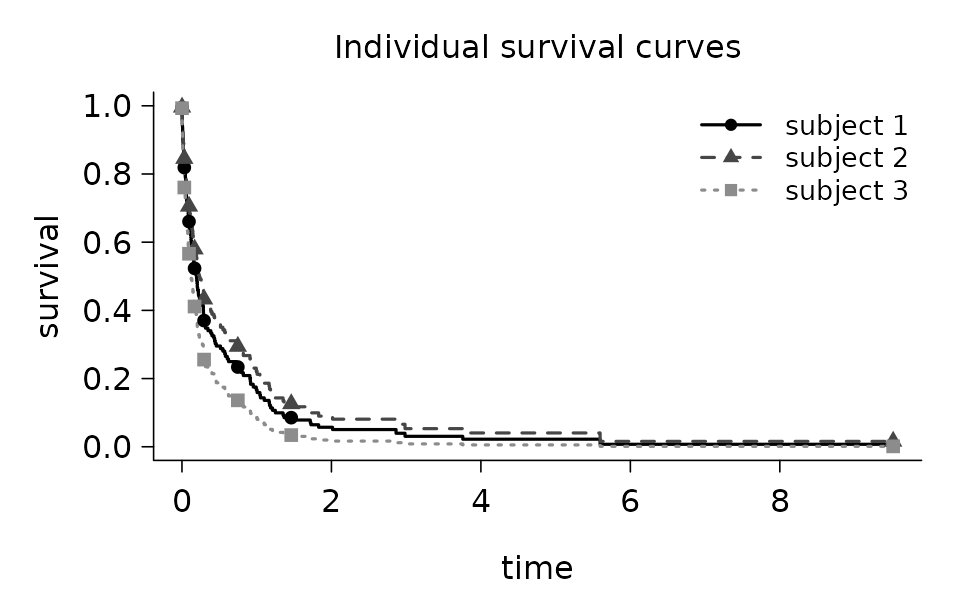

To visualize how a selected variable affects the predicted survival curve, feature_effects_on_survival() evaluates the model on a set of “profile” subjects where all covariates are fixed at their column means except the chosen feature, which varies across several values. By default, the function uses four empirical quantiles of the feature, or all distinct values for small categorical or ordinal variables. The result can be passed directly to plot_survival_curves(). Only variables in the selected support can be queried.

fx <- feature_effects_on_survival(fit_cox, idx = "gene_1")
plot_survival_curves(fx)

A custom grid of values can also be supplied explicitly through the values argument:

fx <- feature_effects_on_survival(fit_cox,
                                  idx    = "gene_3",
                                  values = c(-2, -1, 0, 1, 2))
plot_survival_curves(fx)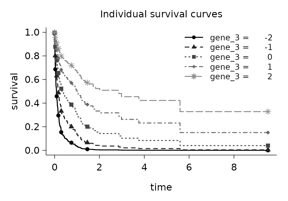

Assessing a fit

Once a model has been trained, assess() reports a compact set of out-of-sample metrics tailored to the distribution. It accepts a fit, a new design matrix, and the corresponding response, and returns a two-column data.frame with columns metric and value:

data(QuickStartExample)
X <- QuickStartExample$X
y <- QuickStartExample$y
fit <- pic(X, y)

assess(fit, newx = X, newy = y)

##  metric     value
##     MSE 1.8231585
##     MAE 1.0851878
##      R2 0.5900742

The metrics depend on the distribution/family:

Family	Metrics reported
Gaussian	MSE, MAE, R²
Binomial	accuracy, AUC, deviance
Poisson	MSE, MAE, deviance
Exponential	MSE, MAE, deviance
Gumbel	MSE, MAE, deviance
Cox	C-index, partial log-likelihood

For Cox fits, newy must be a two-column matrix (time, event), the same format used at training:

data(CoxExample)
fit_cox <- pic(CoxExample$X, CoxExample$y, family = "cox")
assess(fit_cox, newx = CoxExample$X, newy = CoxExample$y)

##                  metric     value
##                 c_index 0.8354248
##  partial_log_likelihood 2.5264204

A note on bias and refitting

A word of caution when interpreting the predictive metrics: by default pic() is called with relax = FALSE, so the reported coefficients still carry the shrinkage induced by the penalty. This is particularly pronounced with the LASSO (penalty = "lasso"), whose bias on non-zero coefficients does not vanish even as the signal grows. SCAD and MCP reduce this effect but the residual bias is still non-negligible for moderate signals.

When the goal is prediction quality, the safest pattern is to refit on the selected support without penalization. Two ways:

Call pic() with relax = TRUE. After the regularized path converges, an unpenalized refit is run on the selected variables, yielding debiased coefficients that are immediately usable for prediction.
Manually re-fit on the subset X[, fit$selected] with the estimator of your choice.

fit_relax <- pic(X, y, relax = TRUE)
assess(fit_relax, newx = X, newy = y)

##  metric     value
##     MSE 0.7631608
##     MAE 0.6993721
##      R2 0.8284080

Support-recovery diagnostics

In a simulation setting where the true active set is known, the optional true_features argument appends four support-recovery metrics to the output: the indicator exact_recovery (1 if the selected support equals the truth), the true-positive rate (tpr, sensitivity), the false-discovery rate (fdr), and the F1 score combining both. Names or integer positions are accepted:

true_active <- paste0("gene_", 1:5)
assess(fit, newx = X, newy = y, true_features = true_active)

##          metric     value
##             MSE 1.8231585
##             MAE 1.0851878
##              R2 0.5900742
##  exact_recovery 1.0000000
##             tpr 1.0000000
##             fdr 0.0000000
##              f1 1.0000000

Diagnostics

picreg exposes two complementary diagnostic tools to assess the behavior of the PIC procedure: support-recovery curves under a sparse-signal Monte Carlo design (phase_transition()), and the asymptotic behavior of the PDB parameter itself in n (pdb_asymptotic()).

Phase transition curves

phase_transition() quantifies, by Monte Carlo, the probability that pic() recovers exactly the true active set as the sparsity level s of the underlying signal varies between 0 and s_max. For each s in the grid, m datasets are generated under the chosen distribution/family with s uniformly random active variables; the function then reports three metrics — exact recovery, true-positive rate, and false-discovery rate — averaged over the replications.

The example below uses a small Monte Carlo size and two configurations. Several penalties can also be requested in a single call (penalty = c("lasso", "scad", "mcp")). Parallel execution over the m replications is enabled with parallel = TRUE.

pt <- phase_transition(
  n        = c(50, 100),
  p        = c(100, 100),
  type     = "gaussian",
  s_max    = 20,
  m        = 100,
  penalty  = c("lasso", "scad"),
  parallel = TRUE
)
plot(pt)

The curves report the probability of exact support recovery: for each configuration the chance that pic() selects precisely the s active variables. The same call accepts metric = "tpr" or metric = "fdr" in the plot method to inspect the true-positive rate or the false-discovery rate.

plot(pt, metric = "fdr")

Asymptotic behavior of the pivotal statistic \Lambda

pdb_asymptotic() runs the three methods for the calculation of \lambda_\alpha^{\mathrm{PDB}} - mc_exact, mc_gaussian, analytical - across a grid of sample sizes n, on a fixed dimensionality p. The result allows one to visualize both the agreement between methods and the rate at which \lambda_\alpha^{\mathrm{PDB}} changes with n. The filled grey histogram is the simulated mc_exact; the dashed step curve overlays the distribution sampled from the CLT Gaussian approximation (mc_gaussian); the solid navy line marks \hat\lambda^{\mathrm{PDB}}_\alpha as estimated by mc_exact, and the dotted vertical line shows the closed-form Bonferroni bound (analytical).

as_ <- pdb_asymptotic(
  n_grid = c(20, 50, 100, 200),
  p      = 200,
  type   = "binomial",
  n_simu = 2000L
)

plot(as_)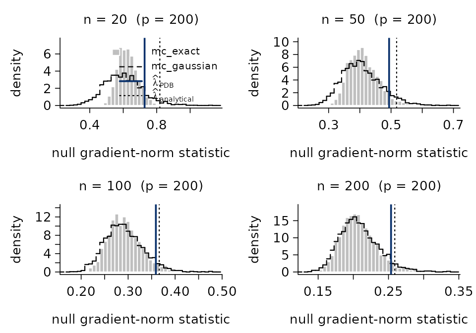

Comparison with other packages

A widely used package for penalized linear regression in the R ecosystem is glmnet (Friedman, Hastie & Tibshirani). glmnet chooses \lambda by cross-validation, which requires fitting a full regularization path and then refitting at the CV-selected value - typically 100 fits. picreg selects \lambda_\alpha^{\mathrm{PDB}} in closed form from the design alone and fits once. More fundamentally, cross-validation tunes \lambda to minimize predictive error, which is not the same objective as recovering the true support; picreg instead calibrates \lambda specifically for support recovery, and therefore tends to recover the active set more accurately. These two targets are fundamentally different - and picreg’s answer is closer to the one practitioners actually want when they ask for “feature selection”

Support recovery on a small Gaussian benchmark

A direct illustration on a sparse Gaussian design. We simulate n = 100 observations, p = 100 covariates, with s = 5 truly active variables (the first five) carrying coefficient 3 and independent standard-Gaussian noise:

set.seed(1)
n <- 100; p <- 100; s <- 5
X <- matrix(rnorm(n * p), n, p)
beta <- numeric(p)
beta[1:s] <- 3
y <- as.numeric(X %*% beta + rnorm(n))
true_support <- seq_len(s)

Three selectors are then run on this single draw: picreg (\ell_1 and \widehat{\lambda}^{\mathrm{PDB}}), cv.glmnet with the prediction-optimal lambda.min, and cv.glmnet with the sparser lambda.1se heuristic.

rbind(
  cbind(method = "picreg (lasso)",         metrics(sel_pic, true_support)),
  cbind(method = "cv.glmnet (lambda.min)", metrics(sel_min, true_support)),
  cbind(method = "cv.glmnet (lambda.1se)", metrics(sel_1se, true_support))
)

##                   method selected exact_recovery
## 1         picreg (lasso)        5           TRUE
## 2 cv.glmnet (lambda.min)       17          FALSE
## 3 cv.glmnet (lambda.1se)        7          FALSE

On this small simulation, picreg typically recovers the five true variables exactly. cv.glmnet recovers them too, but with a handful of additional spurious selections - a well-documented behavior of CV-tuned \ell_1: the chosen lambda.min minimizes prediction error, which usually sits below the support-recovery threshold, so a few noise features sneak in. Using lambda.1se generally produces a sparser model with fewer false positives. However, this choice remains somewhat ad hoc: it is a heuristic designed to favor parsimony rather than a principled calibration specifically targeting support recovery.

A phase transition view

The same effect can be quantified across a grid of sparsity levels by Monte Carlo. We generate Gaussian designs of size n = p = 100 with s \in \{0, 1, \ldots, 12\} active variables (true coefficient magnitude 3, random signs, Gaussian noise), and for each s we report the empirical probability of exact recovery of the active set over m = 100 replications.

A note on speed

A common (and reasonable) concern when leaving glmnet is the runtime. The honest summary first, then a few benchmarks.

For picreg, the actual fit (the FISTA path) is very fast - typically faster than glmnet, because glmnet performs K-fold cross-validation under the hood and thus fits the model on the order of K \times n_\lambda times (typically K=10 folds \times a n_\lambda=100-point grid). The dominant cost in picreg is in fact the computation of \lambda_\alpha^{\mathrm{PDB}} itself, which scales with n:

When n is moderate (say up to a few thousand), even the most accurate "mc_exact" selector is cheap and the whole pipeline finishes very fast.
When n becomes very large, the "mc_exact" Monte Carlo dominates the runtime. In that regime, switching to "mc_gaussian" or "analytical" gives essentially the same \widehat{\lambda} at a tiny fraction of the cost (see the Asymptotic behavior of the selector section), so picreg remains very competitive - often faster than a full CV pass.
For Gaussian designs, glmnet is very fast. Its Fortran coordinate-descent backend on the squared loss is extremely well optimized. picreg runs FISTA on the square-root LASSO loss, which is structurally more expensive per iteration (no closed-form per-coordinate step). On Gaussian benchmarks picreg is therefore slower per fit, although the CV overhead on the glmnet side closes the gap in an end-to-end “fit + select” comparison.

X <- matrix(rnorm(1e4 * 200), 1e4, 200)
Y <- rnorm(1e4)

system.time(pic(X, Y))

##    user  system elapsed 
##   1.238   0.104   1.404

system.time(pic(X, Y, lambda_method = "analytical"))

##    user  system elapsed 
##   0.188   0.023   0.212

system.time(cv.glmnet(X, Y))

##    user  system elapsed 
##   0.998   0.052   1.054

For the other distributions/families, the difference shrinks or even flips: glmnet’s coordinate descent on non-Gaussian likelihoods requires inner Newton-IRLS iterations, while picreg’s FISTA handles them with a single sweep. Combined with the absence of CV, picreg is usually competitive or faster.

X <- matrix(rnorm(1e4 * 200), 1e4, 200)
Y <- rbinom(1e4, size = 1, prob = 0.5)

system.time(pic(X, Y, family = "binomial"))

##    user  system elapsed 
##   1.805   0.115   1.941

system.time(pic(X, Y, family = "binomial", lambda_method = "analytical"))

##    user  system elapsed 
##   0.189   0.023   0.213

system.time(cv.glmnet(X, Y, family = "binomial"))

##    user  system elapsed 
##   3.191   0.084   3.377

Maxime van Cutsem

Sylvain Sardy

June 04, 2026