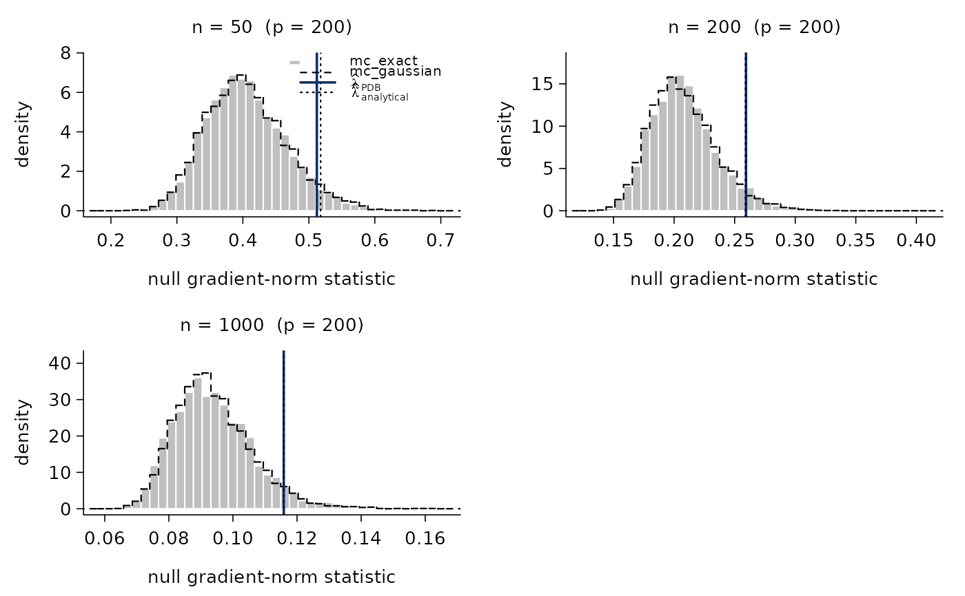
Asymptotic behavior of the PDB null distribution.

For each n in n_grid, draws a standardized Gaussian design matrix of shape (n, p) and computes the null gradient-norm statistic via the three available selectors: "mc_exact", "mc_gaussian", and "analytical". Stores the simulated Monte Carlo statistics and the three resulting \(\hat\lambda\) values per n.

Usage

pdb_asymptotic(
  n_grid,
  p,
  type = c("gaussian", "binomial", "poisson", "exponential", "gumbel", "cox"),
  alpha = 0.05,
  n_simu = 5000L,
  verbose = FALSE
)

Arguments

n_grid: Integer vector of sample sizes to evaluate.
p: Number of features (scalar integer).
type: Family name: "gaussian", "binomial", "poisson", "exponential", "gumbel", or "cox".
alpha: Nominal level used for the (1 - alpha) quantile.
n_simu: Monte Carlo size for each selector.
verbose: Logical; if TRUE, prints a one-line progress message per n.

Value

An object of class c("pic.pdb_asymptotic", "pic.diagnostic").

n_grid, p, type, alpha, n_simu: Configuration.
stats_exact, stats_gaussian: Lists of length length(n_grid) where each element is a numeric vector of length n_simu containing the simulated null statistics from the corresponding selector.
lambda_exact, lambda_gaussian, lambda_analytical: Numeric vectors of length length(n_grid) - the (1 - alpha) quantile under each selector at each n.
call: The call.

Details

The intended use is to visualize the convergence of the exact family-specific null distribution to the Gaussian approximation as n grows — i.e., to check empirically that mc_gaussian is a valid substitute for mc_exact in the asymptotic regime.

Examples

as_ <- pdb_asymptotic(n_grid = c(50, 200, 1000),
                      p = 200, type = "poisson")
plot(as_)